Fixed effects model
In econometrics and statistics, a fixed effects model is a statistical model that represents the observed quantities in terms of explanatory variables that are treated as if the quantities were non-random. This is in contrast to random effects models and mixed models in which either all or some of the explanatory variables are treated as if they arise from the random causes. Often the same structure of model, which is usually a linear regression model, can be treated as any of the three types depending on the analyst's viewpoint, although there may be a natural choice in any given situation.
In panel data analysis, the term fixed effects estimator (also known as the within estimator) is used to refer to an estimator for the coefficients in the regression model. If we assume fixed effects, we impose time independent effects for each entity that are possibly correlated with the regressors.
Contents |
Qualitative description
Such models assist in controlling for unobserved heterogeneity when this heterogeneity is constant over time and correlated with independent variables. This constant can be removed from the data through differencing, for example by taking a first difference which will remove any time invariant components of the model.
There are two common assumptions made about the individual specific effect, the random effects assumption and the fixed effects assumption. The random effects assumption (made in a random effects model) is that the individual specific effects are uncorrelated with the independent variables. The fixed effect assumption is that the individual specific effect is correlated with the independent variables. If the random effects assumption holds, the random effects model is more efficient than the fixed effects model. However, if this assumption does not hold (i.e., if the Durbin–Watson test fails), the random effects model is not consistent.
Quantitative description
Formally the model is

where  is the dependent variable observed for individual
  at time
 is the time-variant regressor,
  is the time-invariant regressor,
  is the unobserved individual effect, and
  is the error term. could represent motivation, ability, genetics (micro data) or historical factors and institutional factors (country-level data).
The two main methods of dealing with are to make the random effects or fixed effects assumption:
1. Random effects (RE): Assume is independent of  or
or 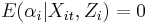 . (In some biostatistical applications, are predetermined,
  and
and  would be called the population effects or "fixed effects", and the individual effect or "random effect" is often denoted
  .)
.)
2. Fixed effects (FE): Assume is not independent of . (There is no equivalent conceptualization in biostatistics; a predetermined cannot vary, and so cannot be probabilistically associated with the random .)
To get rid of individual effect  a differencing or within transformation (time arranging) is applied to the data and then is estimated via Ordinary Least Squares (OLS). The most common differencing methods are:
1. Fixed effects (FE) model: 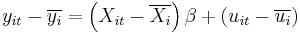 where
where  and
and  .
.
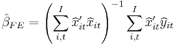
where 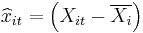 and
and 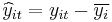
2. First difference (FD) model: 
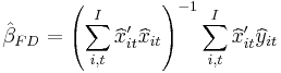
where 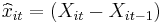 and
and 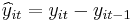
3. Long difference (LD) model: 
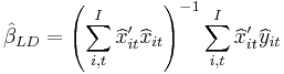
where 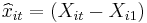 and
and 
Another common approach to removing the individual effect is to add a dummy variable for each individual . This is numerically, but not computationally, equivalent to the fixed effect model and only works if  the number of time observations per individual, is much larger than the number of individuals in the panel.
A common misconception about fixed effect models is that it is impossible to estimate  the coefficient on the time-invariant regressor. One can estimate using Instrumental Variables techniques.
Let 
We can't use OLS to estimate from this equation because is correlated with (i.e. there is a problem with endogeneity from our FE assumption). If there are available instruments one can use IV estimation to estimate or use the Hausman–Taylor method.
Equality of Fixed Effects (FE) and First Differences (FD) estimators when T=2
The fixed effects estimator is:
![{FE}_{T=2}= \left[ (x_{i1}-\bar x_{i}) (x_{i1}-\bar x_{i})' %2B
(x_{i2}-\bar x_{i}) (x_{i2}-\bar x_{i})' \right]^{-1}\left[
(x_{i1}-\bar x_{i}) (y_{i1}-\bar y_{i}) %2B (x_{i2}-\bar x_{i}) (y_{i2}-\bar y_{i})\right]](/2012-wikipedia_en_all_nopic_01_2012/I/a54aad83c5652aef82b0f5265234e1d5.png)
Since each  can be re-written as
  , we'll re-write the line as:
![{FE}_{T=2}= \left[\sum_{i=1}^{N} \dfrac{x_{i1}-x_{i2}}{2} \dfrac{x_{i1}-x_{i2}}{2} ' %2B \dfrac{x_{i2}-x_{i1}}{2} \dfrac{x_{i2}-x_{i1}}{2} ' \right]^{-1} \left[\sum_{i=1}^{N} \dfrac{x_{i1}-x_{i2}}{2} \dfrac{y_{i1}-y_{i2}}{2} %2B \dfrac{x_{i2}-x_{i1}}{2} \dfrac{y_{i2}-y_{i1}}{2} \right]](/2012-wikipedia_en_all_nopic_01_2012/I/0caa1de06b30fe19509804cf176be863.png)
![= \left[\sum_{i=1}^{N} 2 \dfrac{x_{i2}-x_{i1}}{2} \dfrac{x_{i2}-x_{i1}}{2} ' \right]^{-1} \left[\sum_{i=1}^{N} 2 \dfrac{x_{i2}-x_{i1}}{2} \dfrac{y_{i2}-y_{i1}}{2} \right]](/2012-wikipedia_en_all_nopic_01_2012/I/c47024fc0a3107b7fdea0fddcfcb019a.png)
![= 2\left[\sum_{i=1}^{N} (x_{i2}-x_{i1})(x_{i2}-x_{i1})' \right]^{-1} \left[\sum_{i=1}^{N} \frac{1}{2} (x_{i2}-x_{i1})(y_{i2}-y_{i1}) \right]](/2012-wikipedia_en_all_nopic_01_2012/I/9f20aeea969fdac4ed1318a910b0c9f9.png)
![= \left[\sum_{i=1}^{N} (x_{i2}-x_{i1})(x_{i2}-x_{i1})' \right]^{-1} \sum_{i=1}^{N} (x_{i2}-x_{i1})(y_{i2}-y_{i1}) ={FD}_{T=2}](/2012-wikipedia_en_all_nopic_01_2012/I/16722f237709d94cded72624aef9b7ec.png)
Thus the equality is established.
Hausman–Taylor method
Need to have more than one time-variant regressor ( ) and time-invariant regressor (
 ) and at least one and one that are uncorrelated with .
Partition the and variables such that ![\begin{array}
[c]{c}
X=[\underset{TN\times K1}{X_{1it}}\vdots\underset{TN\times K2}{X_{2it}}]\\
Z=[\underset{TN\times G1}{Z_{1it}}\vdots\underset{TN\times G2}{Z_{2it}}]
\end{array}](/2012-wikipedia_en_all_nopic_01_2012/I/7714a62ab13789367ece34ab00872c2f.png) where
where  and
and  are uncorrelated with . Need
  .
.
Estimating via OLS on  using
using  and
and  as instruments yields a consistent estimate.
Testing FE vs. RE
We can test whether a fixed or random effects model is appropriate using a Hausman test.
 :
: 
 :
: 
If is true, both  and
and  are consistent, but only is efficient. If is true, is consistent and is not.


![\widehat{HT}=T\widehat{Q}^{\prime}[Var(\widehat{\beta}_{FE})-Var(\widehat
{\beta}_{RE})]\widehat{Q}\sim\chi_{K}^{2}](/2012-wikipedia_en_all_nopic_01_2012/I/5a25cf14a841cccba1f549d4c41d434b.png) where
where 
The Hausman test is a specification test so a large test statistic might be indication that there might be Errors in Variables (EIV) or our model is misspecified. If the FE assumption is true, we should find that 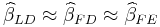 .
.
A simple heuristic is that if  there could be EIV.
Steps in Fixed Effects Model for sample data
- Calculate group and grand means
- Calculate k=number of groups, n=number of observations per group, N=total number of observations (k x n)
- Calculate SS-total (or total variance) as: (Each score - Grand mean)^2 then summed
- Calculate SS-treat (or treatment effect) as: (Each group mean- Grand mean)^2 then summed x n
- Calculate SS-error (or error effect) as (Each score - Its group mean)^2 then summed
- Calculate df-total: N-1, df-treat: k-1 and df-error k(n-1)
- Calculate Mean Square MS-treat: SS-treat/df-treat, then MS-error: SS-error/df-error
- Calculate obtained f value: MS-treat/MS-error
- Use F-table or probability function, to look up critical f value with a certain significance level
- Conclude as to whether treatment effect significantly effects the variable of interest
See also
References
- Christensen, Ronald (2002). Plane Answers to Complex Questions: The Theory of Linear Models (Third ed.). New York: Springer. ISBN 0-387-95361-2.
- "FAQ:What is the between estimator?". http://www.stata.com/support/faqs/stat/xt.html.
- "FAQ: Fixed-, between-, and random-effects and xtreg". http://www.stata.com/support/faqs/stat/xtreg.html.